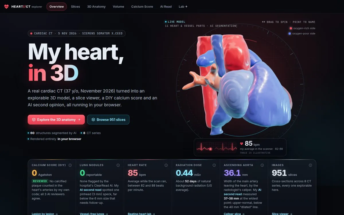
On November 5th I had a cardiac CT, the low-dose “calcium score” kind. The hospital gave me the DICOM export: eight series, 951 slices, and a bundled viewer. I wanted something better than scrolling grey images, so I turned the scan into a website that runs entirely in the browser.
It’s live at cbroker1.github.io/heart-ct-explorer, and the code is at cbroker1/heart-ct-explorer.
The site has seven pages: a beating 3D heart, a slice viewer for every series, a 3D anatomy viewer, a GPU volume renderer, a calcium score I calculated myself from the raw pixels, an AI “second read” of the whole scan, and a lab page driven by my real ECG.
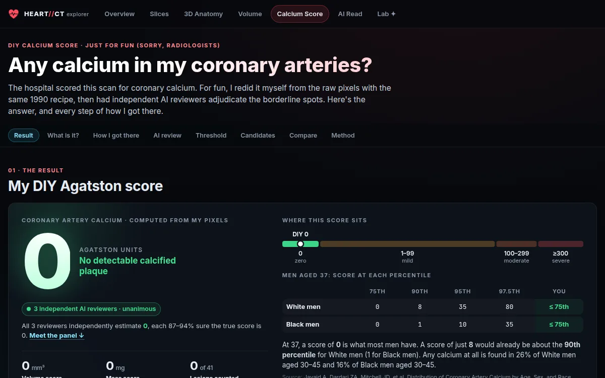
The most interesting part wasn’t the 3D. It was the calcium score. Done the textbook way, my scan scores about 59, which reads as mild coronary artery disease. The real answer is 0, and the work was in proving it.
Not a medical device. This is for curiosity and education. The official radiologist report is what counts.
The pipeline
Everything starts from the DICOM export and goes through eight scripts:
01_convert.py        DICOM → de-identified NIfTI volumes + exam summary
02_segment.sh        TotalSegmentator v2: organs, bones, vessels, pericardium, airways
02b_segment_v1_*.sh  TotalSegmentator v1 cardiac model: the four chambers + myocardium
03_calcium.py        Agatston candidates, review sheets, threshold sweep
04_meshes.py         marching cubes → smoothed, decimated GLB + printable STL
05_web_assets.py     byte-shuffled gzip volumes, label grids, manifest.json
06_ecg.py            digitize the scanner's ECG printout → ecg.json
08_read_report.py    the AI second read → read.json
De-identification happens first: no names, IDs, birth dates or institution survive the conversion. Voxels outside the body are flattened to air, which costs nothing visually and makes the volumes compress far better. The browser downloads them as byte-shuffled, gzipped grids.
TotalSegmentator labels 60 structures, including heart chambers, great vessels, lung lobes, airways, ribs and vertebrae. On a non-contrast scan, blood and heart muscle are nearly the same density, so the chamber boundaries are informed guesses. The site says so wherever it shows them.
The web app
The front end is Vite, React 19 and TypeScript, with three.js and react-three-fiber for the meshes. The two heavy views are written directly against WebGL2.
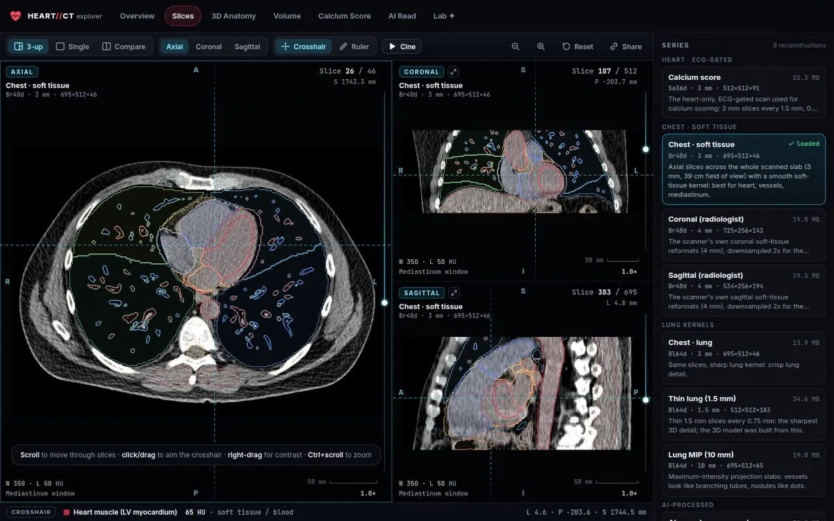
Slices is a multiplanar viewer for all eight series. It has window/level, MIP and MinIP slabs, AI anatomy overlays, a ruler, a side-by-side compare mode, and deep links to any slice and setting.
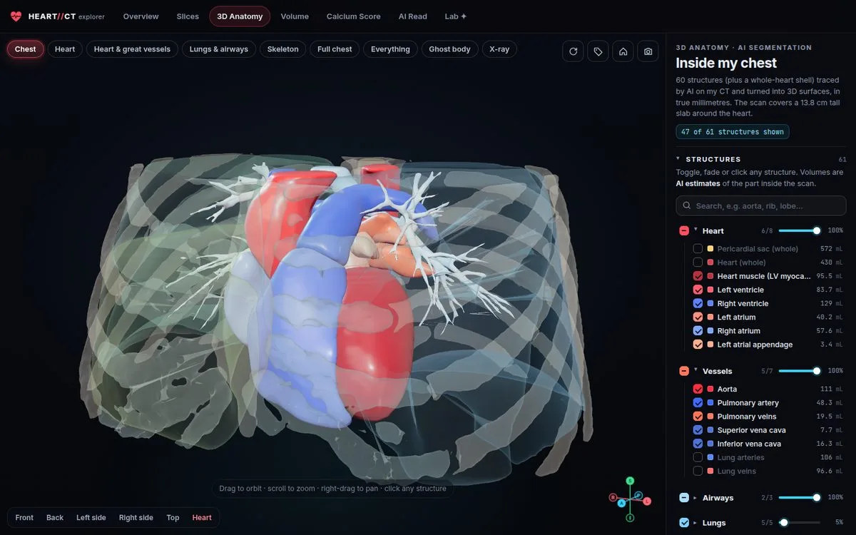
Anatomy 3D shows the segmented structures as meshes, with presets, an explode view, and clipping planes that cut through the real CT underneath.
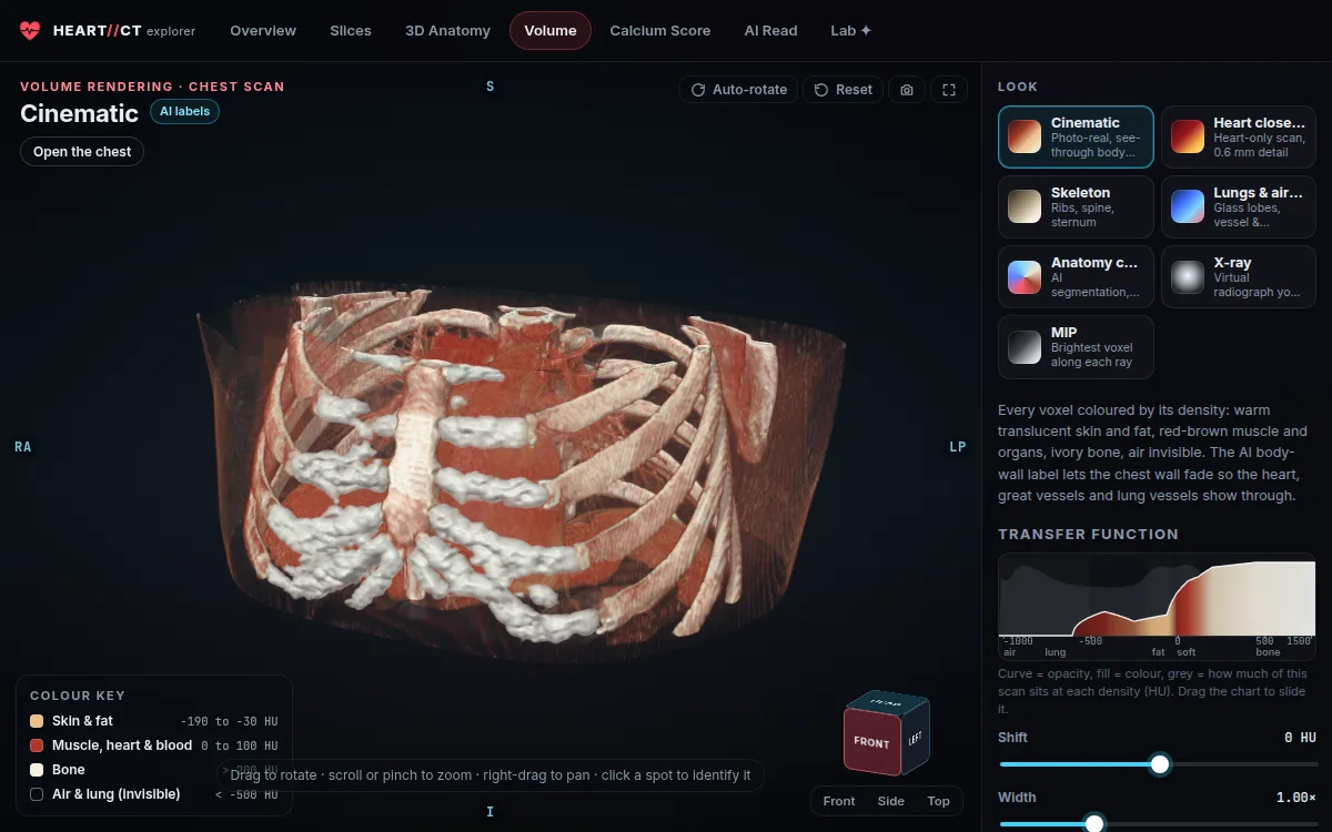
Volume is a GPU ray marcher. Every voxel is colored by its density through an editable transfer function. Presets cover a cinematic look, skeleton, lungs and airways, AI anatomy colors, a virtual X-ray and MIP. The AI body-wall label lets the chest wall fade out so the heart shows through.
The Lab page has the fun extras. The scanner saved my ECG as three printout images, so I digitized the trace from the pixels and used it to drive the beating heart. There’s also a life-size AR heart and a 3D-printable STL of my heart, lungs and ribcage.
A calcium score from raw pixels
A coronary artery calcium (CAC) score counts calcified plaque in the heart’s arteries. The recipe is from Agatston in 1990. Find every spot of at least 1 mm² that reaches 130 HU, and weight each one by its peak density: 1 for 130–199 HU, 2 for 200–299, 3 for 300–399 and 4 for 400 or more. Then multiply each weight by the spot’s area and sum. Zero means no detectable calcified plaque.
I implemented exactly that on the calcium-scoring series (3 mm slices every 1.5 mm, 0.31 mm pixels), searching only inside the pericardium and heart with a 5 mm margin and bone masked out. It found 65 specks on individual slices, which group into 41 candidates in 3D.
That’s where the textbook recipe stops being enough. This is a low-dose scan, and the noise is large: blood inside my heart averages 50 HU with a standard deviation of 18 HU. The 130 HU threshold is only 4.5 standard deviations above blood, so noise alone is expected to clear it. Here’s how the count depends on the threshold:
| Threshold | Specks ≥ 1 mm² | Score if every speck counted |
|---|---|---|
| 100 HU | 943 | 760 |
| 120 HU | 181 | 184 |
| 130 HU | 65 | 59 |
| 140 HU | 20 | 14 |
| 150 HU | 2 | 1 |
| 160 HU | 0 | 0 |
If my code had stopped at 130 HU and counted what it found, it would have printed about 59. That’s “mild” disease, and above the 95th percentile for a man my age. Yet nothing in my heart reaches 200 HU; the brightest voxel inside it on the scoring series is 177 HU.
Where the specks came from
All 41 candidates fall in two thin bands along the body’s long axis, and neither band has anything to do with coronary arteries.
- The bottom edge of the scan, which is the noisiest part of any CT. Candidates #1–13 sit there, in the heart’s apex and the edge of the liver.
- A table-step boundary. This scan was taken step-and-shoot: four table positions of about 34 mm each, joined together. At one join, the inferior heart wall reads 96–99 HU instead of 52–55, a shading shift of about 40 HU. The remaining 28 candidates sit in that band. The scanner’s own coronal reformats show the band as a horizontal stripe.
The upper coronary tree, where calcified plaque actually shows up first (left main, LAD, circumflex, proximal and mid RCA), has zero specks above threshold.
Three reviewers, three different methods
I didn’t want to trust one argument, so I had three independent AI reviewers work on the question in parallel, each with a different method and none seeing the others’ work:
| Reviewer | Method | P(score is 0) |
|---|---|---|
| Candidate adjudicator | Every candidate on its review sheet plus fresh zoomed views at three windows and two reformats | 0.87 |
| Blind sweeper | All 91 slices from scratch, without the candidate list, tracing each coronary territory | 0.94 |
| Cross-reconstruction physicist | A calibrated noise model and 3D simulation against the other reconstructions | 0.90 |
The physicist’s result is the one I find most convincing. Using the measured noise and the measured correlation between neighbouring slices (0.76 at 1.5 mm), its model predicts how many chance specks a scan with no calcium should show:
| Threshold | Predicted from noise alone | Observed |
|---|---|---|
| 130 HU | 61 ± 4 | 65 |
| 140 HU | 21 | 20 |
| 150 HU | 5.8 | 2 |
The noise model accounts for the specks almost exactly. A naive model that treats noise as independent from slice to slice predicts roughly zero, which is the trap. The reviewer also found a useful negative result: comparing reconstructions doesn’t help. Every reconstruction is computed from the same photons, so their noise peaks line up within about 8 HU, and a noise speck looks “confirmed” in all of them.
Another control was that the deep heart muscle, where no coronary artery runs, produces specks at the same rate as the coronary search area.
The reviewers stated the remaining risk plainly: about a 6% chance that candidate #22 is a faint real plaque. If it were, the score would be about 11. The final call was 0, unanimous.
For context: in a 2022 JACC study of nearly 20,000 adults aged 30–45 (Javaid et al.), the 75th percentile score for a 37-year-old man is 0. A score of 0 is what most men my age have.
An AI second read, with a skeptic panel
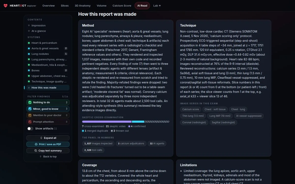
The calcium series is only part of the exam. The other series cover about 14 cm of my chest, from just above the carina down to T12. That takes in the heart, aorta, most of the lungs, the mid thoracic spine, ribs, the liver dome and the top of the spleen. I wanted all of it read systematically, so I set up a review panel modelled on how a radiology department checks itself:
- Eight specialist reviewers: heart; aorta and great vessels; lung nodules; lung parenchyma and airways; mediastinum; bones; upper abdomen and chest wall; technique and artifacts. Each read every relevant series against a radiologist’s checklist and the standard criteria (Fleischner 2017 for nodules, Genant for vertebrae, Framingham reference values for vessel sizes). Each one rendered its own images, took its own measurements in code, and recorded pertinent negatives.
- Three skeptics per finding. Every finding of note, seven in all, went to three independent skeptics with different angles: artifact and anatomy, measurement and criteria, and clinical relevance. Each re-rendered and re-measured from scratch and tried to refute the finding. If a majority refuted it, it was dropped.
- A synthesis pass that looked at the key evidence images directly and wrote the report.
In all, that was 32 agents, about 2,500 tool calls and 1,037 rendered images.
The skeptics earned their place. They threw out 2 of 7 findings:
- “Old healed rib fractures” were a table-seam artifact: the same step-and-shoot joins that faked the calcium specks.
- “Moderate visceral fat” was, on re-measurement, normal.
What survived is reassuring. The heart is normal size (cardiothoracic ratio 0.39), with no pericardial fluid and no valve calcium. The pulmonary artery is normal at about 26 mm, no lymph nodes are enlarged, and there’s no emphysema and no fatty liver. Bone density is healthy. Three small “good to know” notes remain, and none needs follow-up:
- The ascending aorta is 37–38 mm at its widest. That’s upper-normal and below the 40 mm “dilated” line, and a useful baseline.
- One ~3 mm lung micronodule. Fleischner recommends no follow-up below 6 mm for a low-risk person. The hospital’s ClearRead software flagged none.
- Small Schmorl’s nodes (disc imprints) at T9 and T11.
The pattern in the dismissals is the same lesson as the calcium score. On a low-dose sequential scan, the acquisition itself makes things that look like disease. Most of the review’s value came from asking, for each finding, “could the scanner have made this?”
How it was built
I built the whole thing overnight with Claude Code, running agent workflows instead of one long conversation. The clinical read was the 32-agent panel above. The web app came from eight page-builder agents working from a shared spec, followed by a QA pass and an audit of the copy against the data files. The result is about 23,000 lines of TypeScript and 3,900 lines of Python and shell.
The spec did a lot of the work. It fixed the coordinate convention (LPS, everywhere), the data contract between pipeline and app (one manifest.json), and the rules for clinical wording before any page was built. That’s why eight agents writing pages in parallel produced one site instead of eight.
What I’d tell someone doing this
- Get your DICOM. Most hospitals will give you a disc or a download. The raw data is far richer than the PDF report.
- Treat thresholds as hypotheses. A clinical threshold was calibrated on typical scans. On yours, measure the noise first and see what the threshold means in standard deviations.
- Build the null model. “How many of these would pure noise produce?” ended the calcium question faster than any amount of staring at specks.
- Make reviewers argue. Both false findings came from a specialist reviewer and looked plausible. Skeptics told to refute them, re-measuring from scratch, are what caught them.
The scan is mine and I chose to publish it, de-identified. The raw DICOM files and the hospital’s viewer aren’t in the repo. If you have your own calcium-score CT, pipeline/run_all.sh should take you from a DICOMDIR to a working site. The README has the details.